
Selection Scans
Adaptation is a process by which species evolve to become more fit in their environment. The effects of adaptation are apparent in all aspects of life. A particularly deadly example is the adaptation experienced by the HIV virus. If it were not for the high mutation rate in HIV and its resulting resistance to anti-viral drugs, AIDS would not be more dangerous than a mere fever! A better understanding of the dynamics of adaptation in a wide range of organisms including pathogens, insects, plants, and humans will help us to administer appropriate life saving drugs as well as predict the future of bio-diversity.
In this blog post, I give some background about the evolutionary question I address with the H12 and H2/H1 statistics I developed for the detection of adaptation and some of the results of my application of these statistics to D. melanogaster data. The Python and R scripts that I wrote to identify genomic loci under natural selection and to visualize the genomic signatures at loci under selection are available in the Selection Hap Stats GitHub repository.
For further details about H12 and H2/H1, please see our papers in PLoS Genetics:
Garud NR, Messer P, Buzbas E, and Petrov D. “Soft selective sweeps are the primary mode of adaptation in Drosophila.” PLoS Genetics 11: e1005004 (2015).
Garud NR, Messer P, Petrov D. “Detection of hard and soft sweeps from Drosophila melanogaster population genomic data.” PLoS Genetics (2021).
Note: Although the blog post focuses on H12 and H2/H1 from phased data, these same scripts can be used to compute G12, G123, and G2/G1 from unphased data, as featured in our recent paper:
Harris, AM, Garud NR, DeGiorgio M. “Detection and classification of hard and soft sweeps from unphased genotypes by multilocus genotype identity.” Genetics (2018).
Why is adaptation important?
Adaptation is a process in which a species evolves to become more fit in its environment. Virtually all organisms feel the effects of adaptation, especially those experiencing changing environments . For example, the application of pesticides to populations of Drosophila (fruit flies) resulted in the rise in frequency of adaptive mutations conferring pesticide resistance. Another example is the introduction of milk into Northern European diets, resulting in lactase persistence in humans. It is thus essential to identify adaptive events in a wide range of organisms so that we can better understand mechanisms of diseases and various human traits.
What is the genomic signature left behind by adaptation?
Adaptation can leave behind distinct signatures in the genome known as ‘selective sweeps’. Such selective sweeps can be distinguished into hard selective sweeps, where only a single adaptive mutation rises in frequency, or soft selective sweeps, where multiple adaptive mutations at the same locus sweep through the population simultaneously. In both hard and soft selective sweeps, the genetic material surrounding the adaptive mutation, or haplotype, will also elevate in frequency. In a hard sweep, a single haplotype should be present at high frequency, whereas in a soft sweep many haplotypes should be present at high frequencies. Here I present a new statistical method that can identify both hard and soft sweeps in population genomic data.
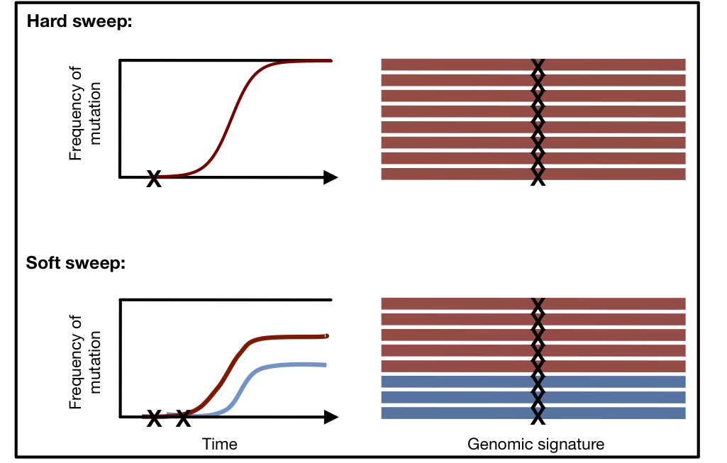
Genomic signatures of hard and soft sweeps arising from one versus multiple mutations. Mutations are indicated by an X. In a hard sweep, only one haplotype will be present at high frequency, whereas in a soft sweep multiple haplotypes will be present at high frequencies (two haplotypes are present at high frequency for the depicted soft sweep). Illustration conceived by Philipp Messer.
A new statistical method to detect hard and soft sweeps
Our statistical test for detecting hard and soft sweeps is based on the reasoning that the increase of haplotype population frequencies in both hard and soft sweeps can be captured using haplotype homozygosity (H1). H1 is a common measure of diversity in population genetics. It is defined as follows:
H1 =Σi=1,…n pi2
where pi is the frequency of the ith most common haplotype in a sample, and n is the number of observed haplotypes. However, as we demonstrate in our paper, H1 has better ability to detect hard sweeps than soft sweeps because there will be one common haplotype at high frequency in a hard sweep as compared to several in a soft sweep. To have a better ability to detect both hard and soft sweeps using homozygosity statistics, we developed modified homozygosity statistic in which the frequencies of the first and the second most common haplotypes are combined into a single frequency.
H12 = (p1 + p2)2 + Σi>2 pi2 = H1 + 2p1p2, .
In order to gain intuition about whether a sweep identified with H12 can be easily generated by hard sweeps versus soft sweeps under several evolutionary scenarios, we developed a new homozygosity statistic, H2/H1, where H2 is haplotype homozygosity calculated using all but the most frequent haplotype:
H2 =Σi>1 pi2 = H1 – p12 .
We expect H2 to be lower for hard sweeps than for soft sweeps because in a hard sweep, only one adaptive haplotype is expected to be at high frequency and the exclusion of the most common haplotype should reduce haplotype homozygosity precipitously. When the sweep is soft, however, multiple haplotypes exist at high frequency in the population and the exclusion of the most frequent haplotype should not decrease the haplotype homozygosity to the same extent. Conversely H1, the homozygosity calculated using all haplotypes, is expected to be higher for a hard sweep than for a soft sweep as we described above. The ratio H2/H1 between the two should thus increase monotonically as a sweep becomes softer, thereby offering a summary statistic that in combination with H12 can be used to test whether the observed haplotype patterns are likely to be generated by hard or soft sweeps.
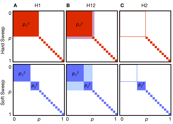
Haplotype homozygosity statistics. Depicted are haplotype frequencies for hard (red) and soft (blue) sweeps. The top row shows incomplete hard sweeps with one prevalent haplotype present in the population at frequency p1, and all other haplotypes present as singletons. The bottom row shows incomplete soft sweeps with one primary haplotype with frequency p1 and a second, less abundant haplotype at frequency p2, with the remaining haplotypes present as singletons. Each edge of the square represents haplotype frequencies ranging from 0 to 1. (A) H1 is the sum of the squares of frequencies of each haplotype in a sample. The total H1 value corresponds to the total colored area. Hard sweeps are expected to have a higher H1 value than soft sweeps. (B) In H12, the first and second most abundant haplotype frequencies in a sample are combined into a single combined haplotype frequency and then homozygosity is recalculated using this revised haplotype frequency distribution. By combining the first and second most abundant haplotypes into a single group, H12 should have more similar power to detect hard and soft sweeps than H1. (C) H2 is the haplotype homozygosity calculated after excluding the most abundant haplotype. H2 is expected to be larger for soft sweeps than for hard sweeps. We ultimately use the ratio H2/H1 to differentiate between hard and soft sweeps as we expect this ratio to have even greater discriminatory power than H2 alone.
A scan for adaptive events in Drosophila data
The data set that we applied our method to is a population genomic data set consisting of 145 Drosophila melanogaster individuals. We applied the H12 and H2/H1 statistics in analysis windows of 400 single nucleotide polymorphisms (SNPs). Take a look at our scan below. We not only recover three known positive controls where adaptation has occurred, but, we also identify several novel adaptive events.
How do we know if an H12 value is significant?
To assess whether the observed H12 values calculated in the data with are unusually high as compared to expectations under neutrality, the highest H12 value expected under realistic demographic models can be estimated using a program such as msms. This critical value of H12 (H12o) can be then used to identify unusually high H12 values relative to neutral expectations.
To call individual sweeps, first all windows with H12 > H12o are identified. Then consecutive windows with H12> H12o are grouped together and considered to belong to the same ‘peak’. The window with the highest H12 value among all windows in a peak is used to represent the H12 values of the entire peak.
In my Selection Hap Stats, I provide Python scripts to calculate H12, H1, and H2 values from data (H12_H2H1.py), identify H12 peaks in the data (H12peakFinder.py), and an R script to visualize the H12 scan (H12_viz.R).
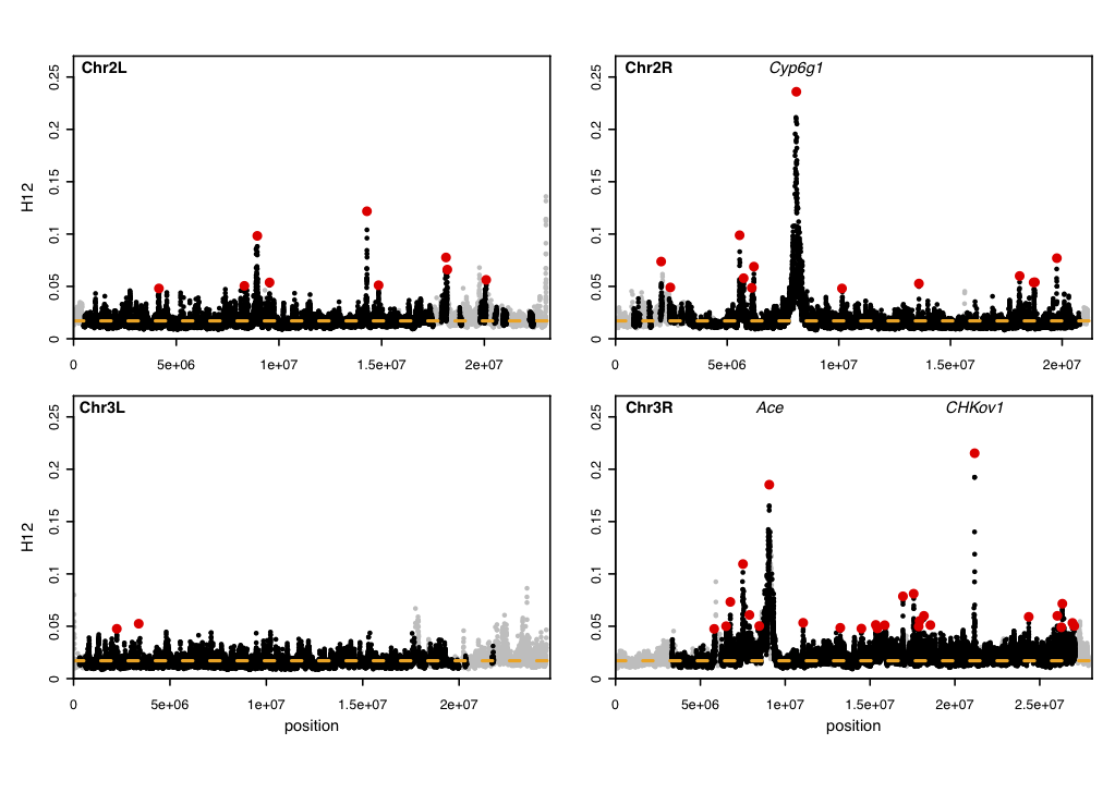
Scan for hard and soft sweeps in Drosophila data. Each data point represents the H12 value calculated in an analysis window of size 400 single nucleotide polymorphisms (SNPs) centered at the particular genomic position. Grey points indicate regions in the genome with low recombination excluded from our analysis because low recombination can generate high H12 values. The orange line represents the highest H12 value calculated under realistic neutral demographic scenarios. Red points highlight the top 50 H12 peaks in the DGRP data relative to the orange line. The positive controls, Ace, CHKov1, and Cyp6g1, are among the top three peaks. This figure was generated with the Python scripts H12_H2H1.py, H12peakfinder.py, and the R script H12_viz.R.
What do individual adaptive events look like in Drosophila data?
To gain intuition as to whether the most extreme candidates for sweeps resemble hard or soft sweeps, we can visually inspect the haplotype frequency spectrum for the analysis window in the H12 peak with the highest H12 value. The R script hapSpectrum_viz.R was written in conjunction with Pleuni Pennings at San Francisco State University (pennings@sfsu.edu).
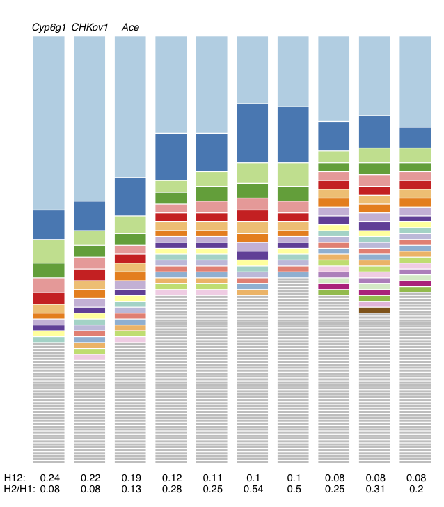
Haplotype frequency spectra for the top 10 H12 peaks highlighted in red in Figure 3. For each peak, the frequency spectrum corresponding to the analysis window with the highest H12 value is plotted. The height of the first bar (light blue) in each frequency spectrum indicates the frequency of the most prevalent haplotype in the sample of 145 individuals, and heights of subsequent colored bars indicate the frequency of the second, third, and so on most frequent haplotypes in a sample. Grey bars indicate singletons. As can be seen, at all peaks there are multiple haplotypes present at high frequency, compatible with signatures of soft sweeps. This figure was generated with hapSpectrum_viz.R.
Haplotype frequency spectra for the top 10 H12 peaks highlighted in red in Figure 3. For each peak, the frequency spectrum corresponding to the analysis window with the highest H12 value is plotted. The height of the first bar (light blue) in each frequency spectrum indicates the frequency of the most prevalent haplotype in the sample of 145 individuals, and heights of subsequent colored bars indicate the frequency of the second, third, and so on most frequent haplotypes in a sample. Grey bars indicate singletons. As can be seen, at all peaks there are multiple haplotypes present at high frequency, compatible with signatures of soft sweeps. This figure was generated with hapSpectrum_viz.R.
A cool way to visualize genomic data and missing data
VisualizeGenomicData.sh generates visualizations of the diversity of the haplotypes in an analysis window and the missing data structure in the analysis window. This visualization can be very informative to gain intuition about the genetic diversity in an analysis window. For example, if the first and second most common haplotypes are very similar to each other, a sweep from standing genetic variation could have occurred. Alternatively, if the first and second haplotypes are more differentiated than expected, then perhaps an adaptive introgression event might have occurred. In addition to viewing the diversity in an analysis window, the visualization can help with understanding the missing data structure. A lot of missing data in an analysis window can result in artificially high H12 values, so such analysis windows should be excluded from any H12 scan. This visual inspection can help identify any spurious artifacts.
 |
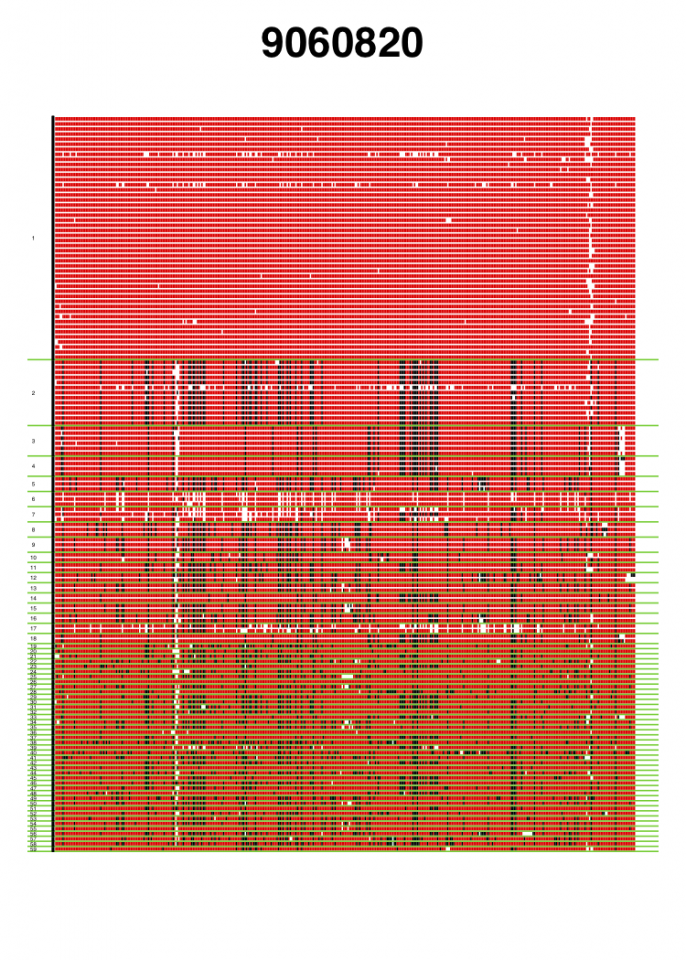 |
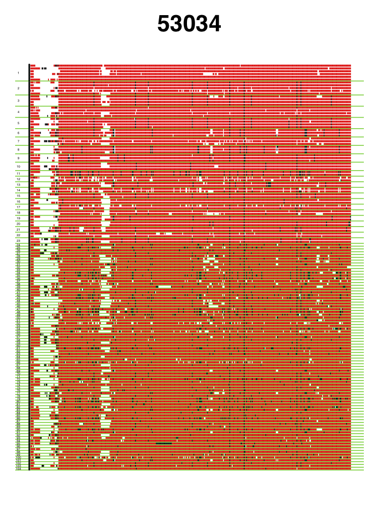
Genomic data visualization for two analysis windows centered around coordinates 9060820 and 53034, respectively. Haplotypes are ordered from most frequent haplotype to least frequent haplotype, and unique haplotypes are separated by a green horizontal line. Numbers of the left side indicate the rank order of the haplotypes in terms of frequency. Red indicates the major allele identified in the most common haplotype. Black indicates any alternate allele from the major allele identified in the first cluster. White indicates missing data. The analysis window centered around coordinate 9060820 coincides with the Ace locus, where a known soft selective sweep has occurred. The analysis window centered around coordinate 53034 is a random analysis window on chromosome 3R of the DGRP data set. These figures were generated with visualizeGenomicData.sh.
So, do the top candidates for adapatation show signatures of hard or soft sweeps?
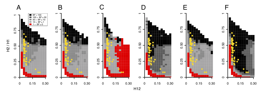
I used an approximate Baysian computation method to determine if a peak’s H12 and H2/H1 values can be most easily generated by hard versus soft sweeps. I performed extensive simulations of hard and soft sweeps under a wide number of evolutionary scenarios and calculated the proportion of simulations with H12 and H2/H1 values closest to the observed values at the top 50 peaks. I then calculated Bayes factors by taking the ratio of the number of soft sweep versus hard simulations with H12 and H2/H1 values matching the data to determine how likely the data is to be generated. In the figure below, the top 50 peaks all have H12 and H2/H1 values that are most easily generated by soft sweeps.
Take-aways from this work:
1. Adaptation is abundant! In our H12 scan, we not only receovered three known cases of adaptation, but we also identified several novel cases.
2. Adaptation commonly leaves behind signatures of soft sweeps, not hard sweeps. This is very surprising given that the classic model of hard sweeps seems to be the exception, not the norm.
3. Adaptation occurs rapidly! Because soft sweeps seem be common, the input of new adaptive mutations must be very high.